Data Source & Purpose of Data Analysis
Data Source: Divvy Bikes license
Purpose of Data Analysis
- How Does a Bike-Share Navigate Speedy Success?
- How can we convert casual riders into members?
- How annual members and casual riders differ?(When and where do they ride?)
If you want to see this project as a HTML document from R Markdown, please click this Link If you want to see this project as a PDF document from R Markdown, please click this Link
1. Prepare Data
1.1 Install Packages
install.packages("tidyverse", repos = "http://cran.us.r-project.org")
library(tidyverse)

install.packages("lubridate", repos = "http://cran.us.r-project.org")
library(lubridate)

install.packages("ggplot2", repos = "http://cran.us.r-project.org")
library(ggplot2)
1.2 Import Data
#Import datasets from Sep 2021 to Aug 2022 and bind them all
filepath <- "data/202109-divvy-tripdata.csv"
new_dataset <- read.csv(filepath)
repeat{
	dateofdata <- as.integer(substr(filepath, 6, 11))+1
	substr(filepath, 6, 11) <- as.character(dateofdata)
	second_import <- read.csv(filepath)
	new_dataset <- rbind(new_dataset, second_import)
	if(dateofdata == 202112){
	filepath <- "data/202201-divvy-tripdata.csv"
	second_import <- read.csv(filepath)
	new_dataset <- rbind(new_dataset, second_import)
	}else if(dateofdata == 202208){
	break
	}
}
2. Process Data
2.1 Create subsets
#Prepare a dataset to inspect its datetime data
dt_dataset <- select(new_dataset, 'ride_id', 'started_at', 'ended_at', 'member_casual')

#Prepare a dataset to inspect geographic data
lc_dataset <- select(new_dataset, 'ride_id', 'start_station_name', 'end_station_name', 'member_casual')
2.2 Organize and Clean Data
- Convert the date columns from character to date type.
- Extract the month column and wday column from the date column.
- Reorder the weekdays, because it's not in the right order.
- Convert the started_at, ended_at columns to time type.
- Calculate the trip duration using the converted time columns.
- Remove bad data which contains negative time difference from trip duration column.
- Deal with missing values.
- Concatenate start and end station names to observe trip routes.
#Data cleaning for dt_dataset

#Convert Character to Date and format to Month and Weekday
dt_dataset$trip_date <- as.Date(dt_dataset$started_at)
dt_dataset$trip_month <- format(as.Date(dt_dataset$trip_date), "%m")
dt_dataset$trip_wday <- format(as.Date(dt_dataset$trip_date), "%a")

#Reorder the weekdays
dt_dataset$trip_wday <- factor(dt_dataset$trip_wday, levels= c("Sun", "Mon", "Tue", "Wed", "Thu", "Fri", "Sat"))

#Convert Datetime to Time datatype, remove rows with negative trip_duration
dt_dataset$trip_stime <- as.POSIXct(dt_dataset$started_at, tz='UTC')
dt_dataset$trip_etime <- as.POSIXct(dt_dataset$ended_at, tz='UTC')

dt_dataset$trip_duration <- difftime(dt_dataset$trip_etime, dt_dataset$trip_stime)
dt_dataset2 <- subset(dt_dataset, trip_duration>0)


#Data Cleaning for lc_dataset

#Deal with missing Values
lc_dataset <- lc_dataset %>%
	filter(start_station_name!=""&end_station_name!="")

#Create trip_route column by concatenating the start and end station names
lc_dataset$trip_route <- paste(lc_dataset$start_station_name, lc_dataset$end_station_name, sep=" - ")

#Create round trip column by inspecting whether start station name equals to end station name or not
lc_dataset$round_trip[lc_dataset$start_station_name==lc_dataset$end_station_name] <- "YES"
lc_dataset$round_trip[lc_dataset$start_station_name!=lc_dataset$end_station_name] <- "NO"
3. Analyze Data
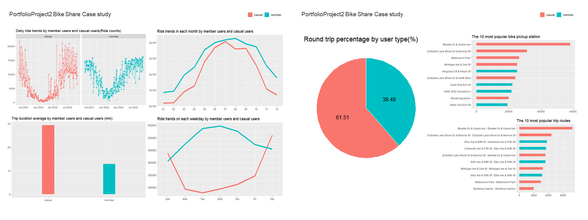
3.1 Daily Bike Ride Trends
#Comparison by the number of daily ride between user types
dt_dataset2 %>%
	group_by(trip_date, member_casual) %>%
	summarize(daily_ride_count=n_distinct(ride_id)) %>%
	ggplot(aes(x = trip_date, y = daily_ride_count, color = member_casual)) +
	geom_point() +
	geom_line(aes(col=member_casual), size=1, alpha=0.4) +
	facet_wrap(~member_casual) +
	labs(title="Daily ride trends by member users and casual users(Ride counts)") +
	theme(axis.title.x=element_blank(), axis.title.y=element_blank(), legend.position="none")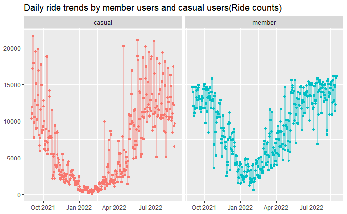
3.2 Bike Ride Tendency by each weekday
#Compare the number of ride by each user type every weekdays
dt_dataset2 %>%
	group_by(trip_wday, member_casual) %>%
	summarise(ride_count_by_weekdays=n_distinct(ride_id)) %>%
	ggplot(aes(x=trip_wday, y=ride_count_by_weekdays, group=member_casual)) +
	geom_line(aes(color=member_casual), size=2) +
	labs(title="Ride trends on each weekday by member users and casual users") +
	theme(axis.title.x=element_blank(), axis.title.y=element_blank(), legend.position="bottom", legend.title = element_blank())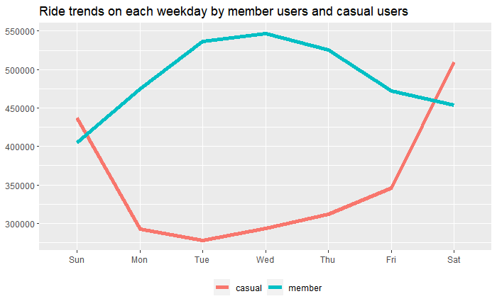
3.3 Bike Ride Tendency by each month
#Compare the number of ride by each user type every months
dt_dataset2 %>%
	group_by(trip_month, member_casual) %>%
	summarise(ride_count_by_months=n_distinct(ride_id)) %>%
	ggplot(aes(x=trip_month, y=ride_count_by_months, group=member_casual)) +
	geom_line(aes(color=member_casual), size=2) +
	labs(title="Ride trends in each month by member users and casual users") +
	theme(axis.title.x=element_blank(), axis.title.y=element_blank(), legend.position="bottom", legend.title = element_blank())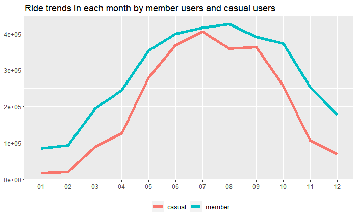
3.4 Average Trip Duration
#Compare the average trip duration between the two user types
dt_dataset2 %>%
	group_by(member_casual) %>%
	summarise(trip_duration_average=mean(as.integer(trip_duration)/60)) %>%
	ggplot(aes(x=member_casual, y=trip_duration_average, fill=member_casual)) +
	geom_bar(stat = "identity", width=0.2) +
	labs(title="Trip duration average by member users and casual users (min)") +
	theme(axis.title.x=element_blank(), axis.title.y=element_blank(), legend.position="none")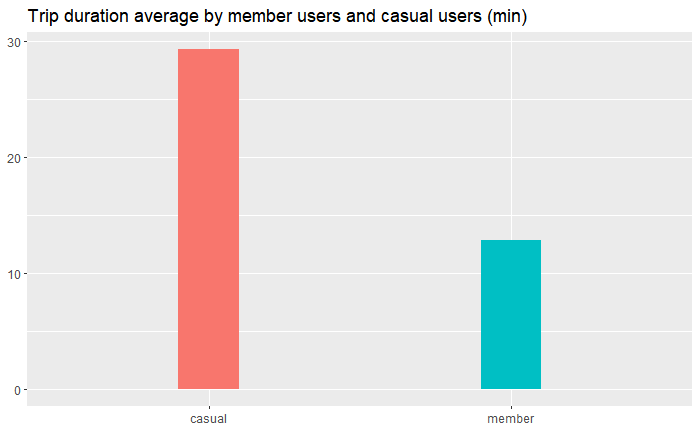
3.5 Round Trip User Proportion
#Create the pie chart to see the proportion of each user type from all the round trips
	lc_dataset %>%
		filter(round_trip=="YES") %>%
		group_by(member_casual) %>%
		summarize(count=n_distinct(ride_id)) %>%
		mutate(percent=count/sum(count)*100) %>%
		ggplot(aes(x = 2, y = percent, fill = member_casual)) +
		geom_bar(stat = "identity", color = "white") +
		coord_polar(theta = "y", start = 0) +
		labs(title="Round trip percentage by user type(%)") +
		geom_text(aes(label = round(percent,2)), position = position_stack(vjust = 0.5), color = "black") +
		theme(axis.text = element_blank(),
			axis.ticks = element_blank(),
			axis.title = element_blank(),
			panel.grid = element_blank(),
			panel.background = element_blank(),
			plot.background = element_blank(),
			legend.position="bottom",
			legend.title = element_blank())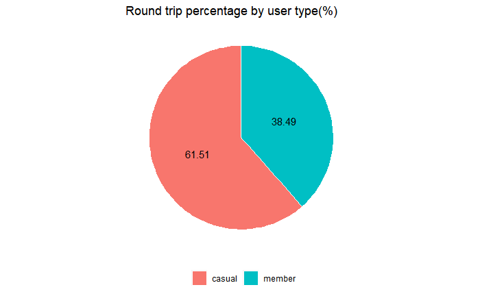
3.6 The 10 Most Popular Trip Route
#Check the 10 most popular trip routes
lc_dataset %>%
	group_by(member_casual, trip_route) %>%
	summarise(count=n_distinct(ride_id)) %>%
	arrange(desc(count), trip_route) %>%
	head(n=10) %>%
	ggplot(aes(x=count, y=reorder(trip_route, count), fill=member_casual)) +
	geom_bar(stat = "identity", width=0.4) +
	labs(title="The 10 most popular trip routes") +
	theme(axis.title.x=element_blank(), axis.title.y=element_blank(), legend.position="bottom", legend.title = element_blank())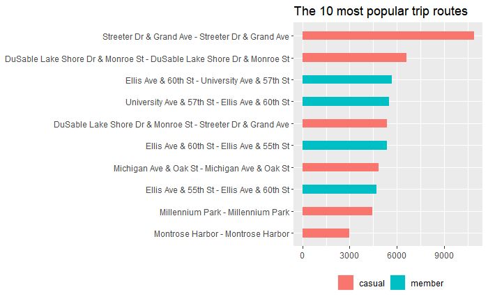
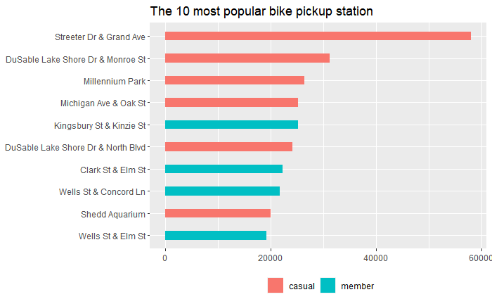
3.7 The 10 Most Popular Pickup Station
#Create the bar chart to see the top 10 popular station to start the trip
lc_dataset %>%
	group_by(start_station_name, member_casual) %>%
	summarize(ride_count=n_distinct(ride_id)) %>%
	arrange(desc(ride_count)) %>%
	head(n=10) %>%
	ggplot(aes(x=ride_count, y=reorder(start_station_name, ride_count), fill=member_casual)) +
	geom_bar(stat = "identity", width=0.4) +
	labs(title="The 10 most popular bike pickup station") +
	theme(axis.title.x=element_blank(), axis.title.y=element_blank(), legend.position="bottom", legend.title = element_blank())